cropdatape provides peruvian agricultural production data from the Agriculture Minestry of Peru (MINAGRI). The first version includes 6 crops: rice, quinoa, potato, sweet potato, tomato and wheat; all of them across 24 departments. Initially, in excel files which has been transformed and assembled using tidy data principles, i.e. each variable is in a column, each observation is a row and each value is in a cell. The variables variables are sowing and harvest area per crop, yield, production and price per plot, every one year, from 2004 to 2014.
Installation
You can install cropdatape directly from CRAN:
install.packages("cropdatape")Or, you can install from GitHub:
# install.packages("devtools")
devtools::install_github("omarbenites/cropdatape")
The cropdatape data frame include 9 variables,
| variable | meaning | units |
|---|---|---|
| crop | crop | - |
| department | deparment or region | - |
| year | year | - |
| month | month | - |
| sowa | sowing area | ha |
| harva | harvested area | ha |
| production | production | t |
| yield | yield | kg/ha |
| pricePlot | price per plot | s/kg |
Usage
Example 1: Filter, grouped and summarize cropdatape data
In this example, we will explore the cropdatape dataset, using three (dplyr) functionlities: filter, group and summarize.
-
filtercrop bysweet potato. -
group_bydepartment column. -
summariseby mean of the sweetpotato yield.
cropdatape package:
#Load cropdatape package
library(cropdatape)
#Load dplyr package to filter and select information
library(dplyr)
cropdatape %>%
      filter(crop == "sweet potato") %>%
      group_by(department, year) %>%
      summarise(yieldMean = mean(yield, na.rm = TRUE))
#> # A tibble: 235 x 3
#> # Groups:   department [?]
#>    department  year yieldMean
#>    <fct>      <dbl>     <dbl>
#>  1 Amazonas    2004      NaN
#>  2 Amazonas    2005     7100.
#>  3 Amazonas    2006     6754.
#>  4 Amazonas    2007     9254.
#>  5 Amazonas    2008    10185.
#>  6 Amazonas    2009     8009.
#>  7 Amazonas    2010     7817.
#>  8 Amazonas    2011     7769.
#>  9 Amazonas    2012     8017.
#> 10 Amazonas    2013     7150.
#> # ... with 225 more rows
Example 2: Plot graphics with ggplot using cropdatape data
This second example we will explore the behaviour of the yield varible grouped by crop, from 2004 till 2014. The crop variable involves 6 crops: potato, quinoa, rice, sweet potato and wheat.
library(cropdatape)
library(ggplot2)
ggplot(cropdatape, aes(x = crop, y = yield)) +
  geom_boxplot(outlier.colour = "hotpink") +
  geom_jitter(position = position_jitter(width = 0.1, height = 0), alpha = 1/4)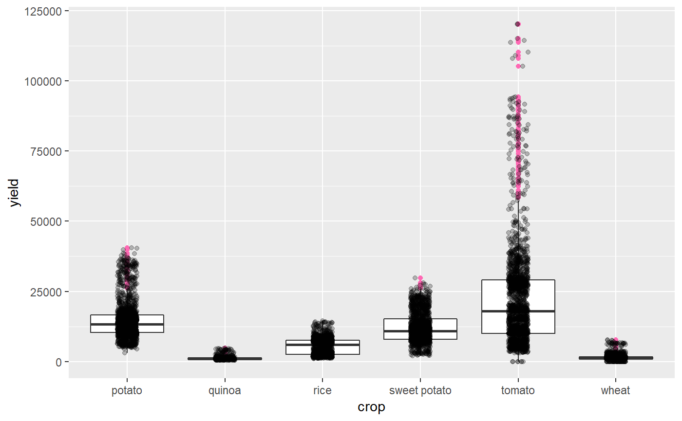
Example 3: Animations with gganimate
To begin with, install the following packages from Github:
#Install first devtools package
#install.packages("devtools")
library(devtools)
install_github("thomasp85/gganimate")
install_github("thomasp85/transformr")
install_github("thomasp85/tweenr")
Then, we will filter all the information related to sweetpotato
library(cropdatape)
library(dplyr)

sp <- cropdatape %>%
      filter(crop == "quinoa", department == "Puno") %>%
      group_by(department, year) %>%
      summarise(sowaMean = mean(sowa,na.rm = TRUE),
                harvaMean = mean(harva, na.rm = TRUE),
                yieldMean = mean(yield, na.rm = TRUE))
Plotting and animating the scatter graph years vs yieldMean
library(gganimate)
library(ggplot2)
library(transformr)
sp$year <- as.integer(sp$year)
yearlbl<- sp$year
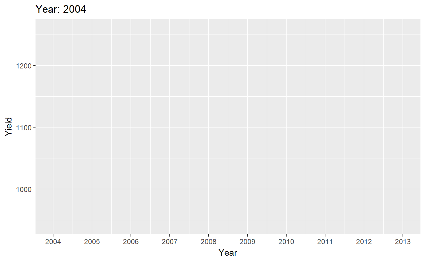
ggplot(sp, aes(year, yieldMean)) +
geom_point(size= 1.5)+
scale_x_continuous(breaks = yearlbl)+
labs(title = 'Year: {frame_time}', x = 'Year', y = 'Yield') +
transition_time(year) +
ease_aes('linear')
Install and emojifonts package:
devtools::install_github("dill/emoGG")
library(emoGG)
Let the animation begins,
library(gganimate)
library(ggplot2)
library(transformr)
sp$year <- as.integer(sp$year)
yearlbl<- sp$year
ggplot(sp, aes(year, yieldMean)) +
  scale_x_continuous(breaks = yearlbl)+
  geom_emoji(emoji="1f360")+
  labs(title = 'Year: {frame_time}', x = 'Year', y = 'Yield') +
  transition_time(year) +
  ease_aes('linear')